Coupled Cluster Monte Carlo

In this tutorial we will run CCMC on the carbon monoxide molecule in a cc-pVDZ basis. For details of the theory see [Thom10] and [Spencer15].

This tutorial only presents the basic options available in a CCMC calculation; for the full range of options see the main documentation.

To perform calculations on a molecular system in HANDE, we need the one- and two- electron integrals in some appropriate basis from an external source. For the calculations in this tutorial, the integrals were calculated using Psi4; input and output files can be found with the files from the calculations herein in the documentation/manual/tutorials/calcs/ccmc subdirectory.

The system definition is exactly the same as for FCIQMC:

sys = read_in {
    int_file = "CO.CCPVDZ.FCIDUMP",
    nel = 14,
    ms = 0,
}

Note that we have not specified an overall symmetry. In this case HANDE uses the Aufbau principle to select a reference determinant.

A CCMC calculation can be run in a very similar way to FCIQMC. As for FCIQMC we can substantially reduce stochastic error by using real amplitudes, which we do for all calculations presented here. The most significant difference from an FCIQMC input is that it is standard to use truncation with CCMC, specified by the ex_level option, (i.e. 2 for CCSD, 3 for CCSDT, etc.). The determination of a plateau and hence a suitable value for target_population is exactly analogous to FCIQMC, as the sign problem is similar between the two methods; we will not discuss it further here. The CCSDTMC calculation can be run using an input file such as:

sys = read_in {
    int_file = "CO.CCPVDZ.FCIDUMP",
    nel = 14,
    ms = 0,
}

ccmc {
    sys = sys,
    qmc = {
        tau = 1e-3,
        mc_cycles = 10,
        nreports = 1e5,
        state_size = -500,
        spawned_state_size = -200,
        init_pop = 1e4,
        target_population = 1e6,
	real_amplitudes = true,
    },
    reference = {
        ex_level = 3,
    },
}

Note the much larger initial population compared to an FCIQMC calculation; if this is too low the correct wavefunction will not be obtained.

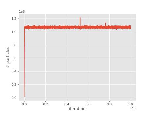
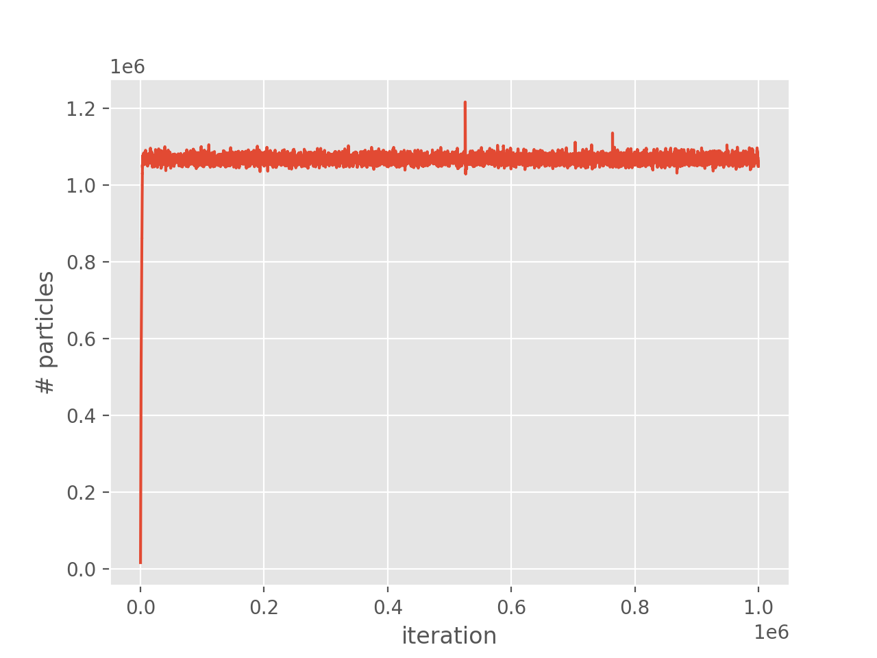
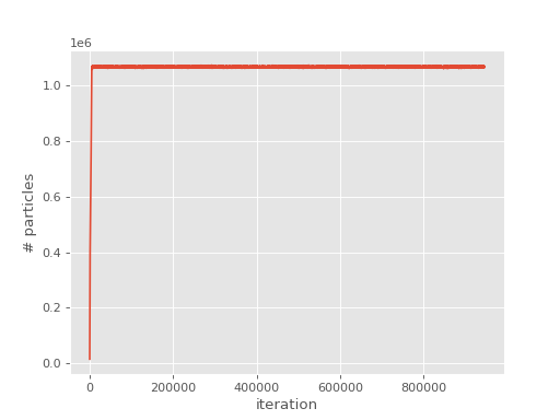
Looking at the output, we see the evolution of the population has a similar form to FCIQMC:

(Source code, png, hires.png, pdf)

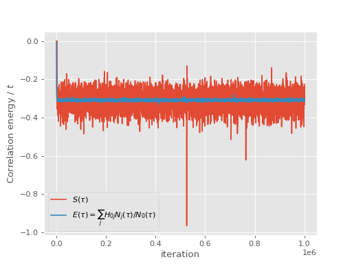
and the shift and projected energy vary about the correlation energy:

(Source code, png, hires.png, pdf)

The output of the calculation can be analysed in exactly the same way as for FCIQMC:

$ reblock_hande.py --quiet --start 100000 co_ccmc.out

giving

Recommended statistics from optimal block size:

                     # H psips \sum H_0j N_j        N_0       Shift Proj. Energy
ccmc/co_ccmc.out  1066600(100)     -6510(10)  21040(40)  -0.3092(6)  -0.30925(7)

Due to the sampling of the wavefunction in CCMC, it is more prone to “blooming” events where many particles are created in a single spawning event than is FCIQMC. Details of blooming during a calculation are reported at the end of the output. It can be seen that significant blooming occurred. This substantially increases the stochastic error, and in particularly severe cases can cause the calculation to not give a correct result due to the instability. These events can be avoided by reducing the timestep, but the timestep required to eliminate them entirely is often prohibitively small. Another way of reducing them is the use of the cluster_multispawn_threshold keyword, whereby large spawning attempts are divided into a number of smaller spawns:

sys = read_in {
    int_file = "CO.CCPVDZ.FCIDUMP",
    nel = 14,
    ms = 0,
}

ccmc {
    sys = sys,
    qmc = {
        tau = 1e-3,
        mc_cycles = 10,
        nreports = 1e5,
        state_size = -500,
        spawned_state_size = -200,
        init_pop = 1e4,
        target_population = 1e6,
	real_amplitudes = true,
    },
    ccmc = {
	cluster_multispawn_threshold = 10,
    },
    reference = {
        ex_level = 3,
    },
}

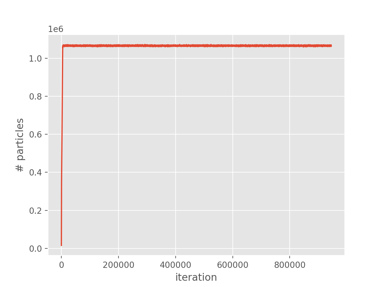
Running as before, and inspecting the output, it can be seen that there are now no blooms. Additionally, plotting the population growth and comparing to the previous plot we see that there are now no spikes in the population:

(Source code, png, hires.png, pdf)

This substantially reduces the stochastic error:

Recommended statistics from optimal block size:

                               # H psips \sum H_0j N_j       N_0       Shift Proj. Energy
ccmc/co_ccmc_multispawn.out  1066160(30)     -11191(1)  36178(7)  -0.3091(1)  -0.30933(3)

The extra spawning causes the calculation to run more slowly, but the reduction in error bars can often more than make up for this.