Density Matrix Quantum Monte Carlo
In this tutorial we will run DMQMC on the 2D Heisenberg model and the uniform electron gas.
The input and output files can be found under the documentation/manual/tutorials/calcs/dmqmc
subdirectory of the source distribution. Knowledge of the terminology and theory given in
[Booth09], [Blunt14] and [Malone15] is assumed.
To begin we will focus on the 6x6 antiferromagnetic Heisenberg model on a square lattice with periodic boundary conditions. The input file for this system is given as
sys = heisenberg {
    lattice = {
        {6, 0},
        {0, 6},
    },
    J = -1.0,
    ms = 0,
}

dmqmc {
    sys = sys,
    qmc = {
        tau = 0.001,
        init_pop = 5e6,
        rng_seed = 19838,
        mc_cycles = 10,
        nreports = 500,
        shift_damping = 0.5,
        target_population = 5e6,
        state_size = -400,
        spawned_state_size = -400,
    },
    dmqmc = {
        beta_loops = 1,
    },
    operators = {
        energy = true,
        excit_dist = true,
    },
}
and is largely analogous to that found in the FCIQMC tutorial. We
refer the reader to the discussion there and the manual for system specific input options.
Note that init_pop here controls the population with which the density matrix at
\(\beta=0\) is sampled. Typically the shift is allowed to vary from the beginning of
a simulation by setting target_pop equal to init_pop. Here we will attempt to run to
a final temperature of \(\beta = 5/J\).
The beta_loops option determines the number of independent simulations over which
observables are averaged, see dmqmc options for more options. The operators table
specifies which observables are to be evaluated in a given simulation. Here only the total
energy is considered, a full list is available in operators options.
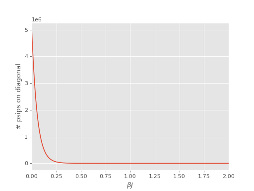
An issue encountered when applying DMQMC to larger systems is that the population on the diagonal (denoted Trace in the output file) decays with increasing \(\beta\) which results in poor estimates for observables. The seriousness of this problem needs to be assessed on a system by system basis and should be tested for as a first step, which we’ll do now.
To do this we set beta_loops to 1 in the input file and run the code as:
$ aprun -B hande.x heisenberg_dmqmc.lua > heisenberg_dmqmc.out
We find that for this system the population on the diagonal does indeed decay to zero rapidly:
(Source code, png, hires.png, pdf)

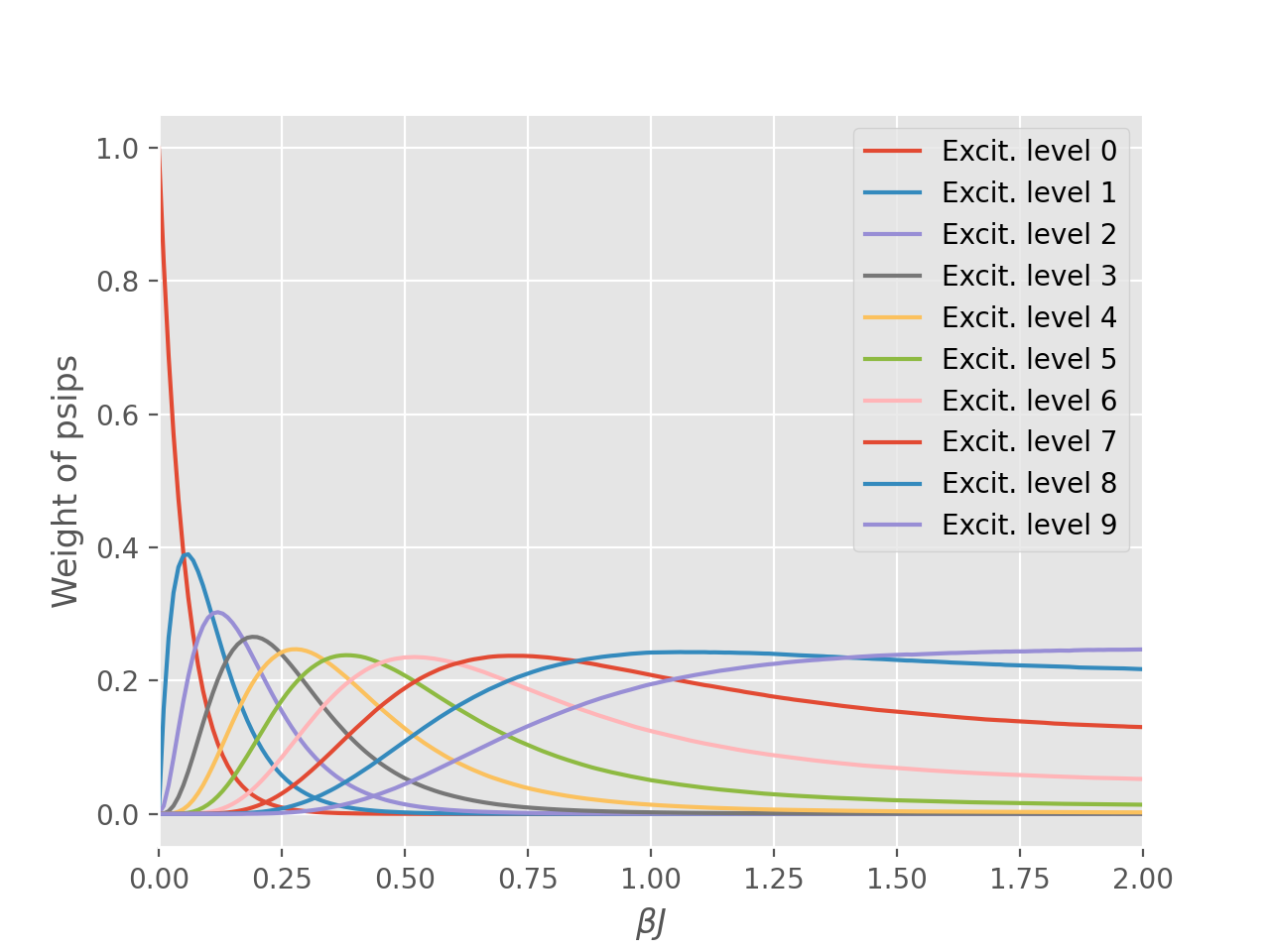
The source of this problem can be investigated by analysing the distribution of psips on
different excitation levels of the density matrix, which was calculated in anticipation of
this result using the excit_dist option in the operators table. Here the excitation
level is defined as the difference between the bra and ket of a density matrix element
i.e., number of spin flips or number of particle-hole pairs for electronic systems.
We see the majority of the total weight is redistributed from the diagonal to highly
excited determinants.
(Source code, png, hires.png, pdf)
To overcome this [Blunt14] invented an unbiased importance sampling scheme to encourage psips to stay on or near the diagonal by penalising spawning moves away from excitation levels. This is sensible as typically the majority of the weight contributing to most physically significant observables originates from the determinants at lower excitation levels which we wish to sample more regularly.
Practically this amounts to first running a calculation with the find_weights
option. This will output importance sampling weights which are appropriate as input for the
production calculation. It is worthwhile to run the calculation for a few beta_loops
to ensure the weights are not fluctuating too much, and also check they don’t fluctuate too
much with the target_population. The algorithm currently tries to ensure that the
number of walkers on each excitation level is roughly constant once the ground state is
thought to have been to be reached. The iteration number where this is deemed to have
been reached is controlled by the find_weights_start option.
For this system we do
$ aprun -B hande.x heisenberg_find_weights.lua > heisenberg_reweighted.out
Here we first run a simulation for 10 beta loops to find the weights and then use the last iteration’s weights as input to the production calculation. This procedure can simplified using lua as seen in the input file.
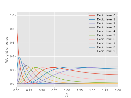
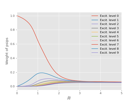
To see what is going on we can copy the weights from the output file and run for a single iteration and again examine the excitation distribution
$ aprun -B hande.x heisenberg_reweight_single.lua > heisenberg_reweight_single.out
and we find that the psips are now more equally distributed among excitation levels:
(Source code, png, hires.png, pdf)
The results of the full reweighted calculation can be analysed using the
finite_temperature_analysis.py script provided in the tools/dmqmc subdirectory:
$ finite_temp_analysis.py heisenberg_reweighted.out > heisenberg_reweighted_block.out
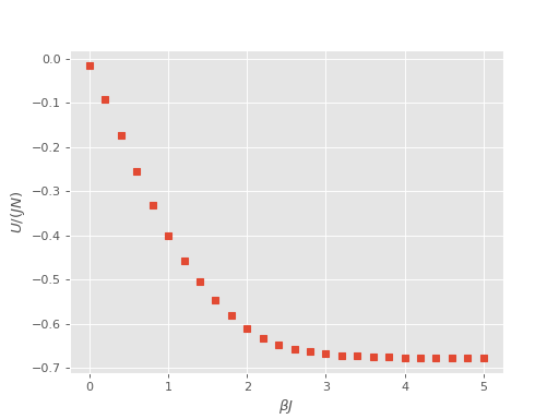
Finally, we can plot the results of the internal energy, \(U\), as a function of temperature:
(Source code, png, hires.png, pdf)

Interaction Picture Density Matrix Quantum Monte Carlo
It turns out that the original formulation of DMQMC can run into problems for moderately weakly interacting systems which are relatively well described by Hartree–Fock theory. An extreme example of this is the uniform electron gas (UEG) especially at higher densities (low \(r_s\)). This issue is largely overcome by switching to the interaction picture which enables us to start from a (temperature dependent) mean-field distribution at \(\tau=0\) ensuring low energy determinants are initially sampled. See [Malone15] for details. For systems with a good mean-field ground state the user should consider using IP-DMQMC.
Most of the running details for IP-DMQMC are the same as for DMQMC, however there are some additional considerations. This is best demonstrated by running a simulation. We will focus on a 7-electron, spin polarised system in 319 plane waves at \(r_s=1\).
Looking at the input file
sys = ueg {
    nel = 7,
    ms = 7,
    sym = 1,
    dim = 3,
    cutoff = 10,
    rs = 1,
}

dmqmc {
    sys = sys,
    qmc = {
        tau = 0.001,
        rng_seed = 7,
        init_pop = 10000,
        mc_cycles = 10,
        nreports = 100,
        target_population = 10000,
        state_size = -200,
        spawned_state_size = -100,
    },
    dmqmc = {
        fermi_temperature = true,
        all_sym_sectors = true,
        beta_loops = 100,
    },
    ipdmqmc = {
        target_beta = 1.0,
        initial_matrix = 'free_electron',
        grand_canonical_initialisation = true,
        symmetric = false,
    },
    operators = {
        energy = true,
    },
}
we see most of the same options are present as for dmqmc. Note that unlike DMQMC where
estimates for the whole temperature range are gathered in a single simulation, in IP-DMQMC
only one temperature value is (directly) accessible, specified by the target_beta
option. We’ve also set the energy scale to be determined by the Fermi energy of the
corresponding (thermodynamic limit) free electron gas so that the temperatures are
interpreted as fractions of the Fermi temperature (here \(\Theta = 0.5\).
all_sym_sectors ensures all momentum symmetry sectors are averaged over. To average
over spin polarisation the all_spin_sectors option must be specified.
Moving on through the ipdmqmc table we’ve set the initial_matrix to be the free
electron density matrix, i.e., Fermi-Dirac like. Additionally we’re using the
grand_canonical_initialisation option to initialise this density matrix (see
[Malone15]). This is the recommended method to initialise the density matrix; the
Metropolis algorithm should only be used for testing.
Finally we will use the asymmetric form of the original IP-DMQMC algorithm by specifying
symmetric to be false. The symmetric algorithm is somewhat experimental but can lead to better
estimates for quantities other that the internal energy especially at lower temperatures.
This is thought to be due to sampling issues at low temperatures where the initial mean field
guess becomes significantly different (in terms of energy scales) to the fully interacting theory.
Symmetrising the equations allows psips to move along rows and which improves sampling.
See [Malone16].
Running the code
$ hande.x ipdmqmc_ueg.lua > ipdmqmc_ueg.out
and analysing the output:
$ finite_temp_analysis.py ipdmqmc_ueg.out > ipdmqmc_ueg_block.out
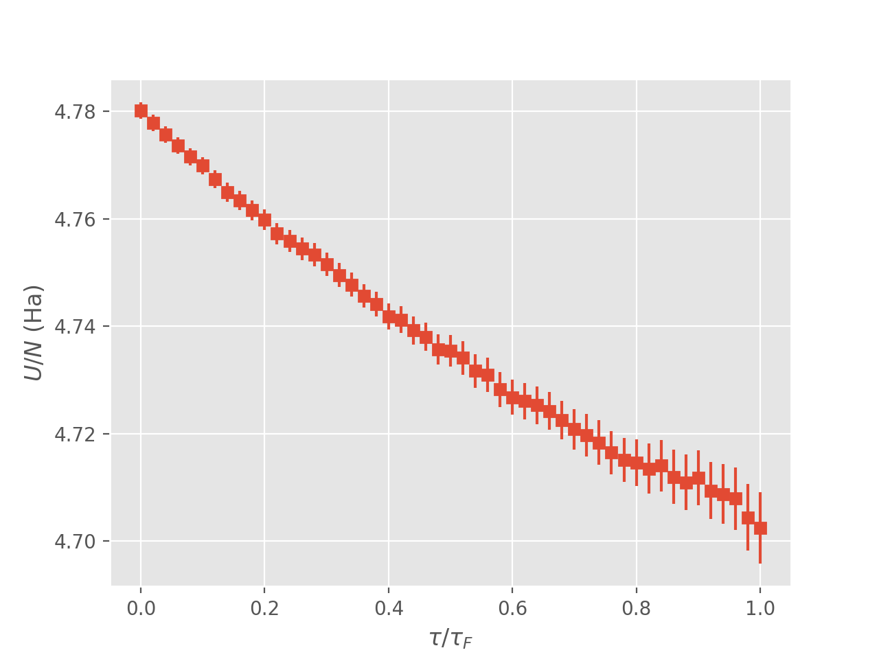
we find
(Source code, png, hires.png, pdf)
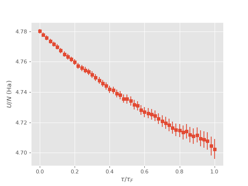
where again only estimates at the final iteration are physical, i.e., when \(\tau=\beta\). Note that the estimates do not contain a Madelung constant.
The initiator approximation can significantly extend the range of applicability of DMQMC
but is somewhat experimental. See the options, in particular initiator_level in the
manual for more discussion. The user should ensure results are meaningful by comparing
answers at various walker populations. See [Malone16] for further discussion.