Semi-Stochastic FCIQMC
In this tutorial we will explain how to run FCIQMC calculations using the
semi-stochastic adaptation to reduce stochastic errors [Petruzielo12]. We
will consider the half-filled 18-site 2D Hubbard model at \(U/t=1.3\),
as previously considered in the basic Full Configuration Interaction Quantum Monte Carlo tutorial. In
particular, we shall begin from the input file presented at the end of the
FCIQMC tutorial, which introduces the use of non-integer psip amplitudes
through the real_amplitudes keyword:
hubbard = hubbard_k {
    lattice = {
        { 3,  3 },
        { 3, -3 },
    },
    electrons = 18,
    ms = 0,
    U = 1.3,
    t = 1,
    sym = 1,
}

fciqmc {
    sys = hubbard,
    qmc = {
        tau = 0.002,
        mc_cycles = 20,
        nreports = 10000,
        init_pop = 100,
        target_population = 4*10^6,
        state_size = -1000,
        spawned_state_size = -100,
        real_amplitudes = true,
    },
}
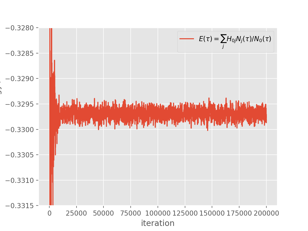
and which results in the following simulation:
(Source code, png, hires.png, pdf)
The semi-stochastic adaptation provides a way to reduce the stochastic noise in such simulations. It does so by choosing a certain subspace (called the deterministic subspace), which is deemed to be most important (in that most of the wave function amplitude resides in this subspace), and performing projection exactly within it. Projection outside the subspace is performed by the usual FCIQMC stochastic spawning.
Thus, we simply need to specify what subspace to use for the exact projection. One way of doing this is by using the scheme of [Blunt15], where the subspace is formed from the determinants on which the largest number of psips reside. We therefore simply need to tell HANDE what iteration to start using the semi-stochastic adaptation, and how many determinants to form the deterministic subspace from.
There are a couple of things to consider when choosing the size of the deterministic space. Firstly, within the deterministic subspace, the Hamiltonian is stored exactly in a sparse form. Therefore, using semi-stochastic does increase memory requirements. The deterministic Hamiltonian storage (and multiplication) is distributed across processing cores, which allows larger subspaces to be used. The other consideration is that, for very large deterministic spaces, and for certain systems (particularly strongly correlated systems), semi-stochastic can slow simulations down slightly. Through investigation (for example, see [Blunt15]), it has been found that a deterministic space of size \(10^4\) allows a very large reduction in stochastic error for most simulations, while not increasing simulation time. We therefore suggest this as a black box subspace size. This is also small enough that the deterministic Hamiltonian can always be stored, even if using only a typical desktop computer.
Note that because semi-stochastic does not usually reduce iteration time much (and sometimes increases it), one should not worry that we do not use semi-stochastic from the first iteration. We are only concerned with reduction in stochastic error from the point where data will be averaged later.
Looking at the above simulation, it appears that the energy has converged by iteration \(2 \times 10^4\). This is not a guarantee that the wave function is also fully converged, but full convergence is not critical – so long as the most important determinants are in the deterministic subspace, then a large reduction in stochastic error will occur. As discussed above, a reasonable deterministic space size is \(10^4\). So, to start using a deterministic space of size \(10^4\) at iteration \(2 \times 10^4\), we modify the above input to the following:
hubbard = hubbard_k {
    lattice = {
        { 3,  3 },
        { 3, -3 },
    },
    electrons = 18,
    ms = 0,
    U = 1.3,
    t = 1,
    sym = 1,
}

fciqmc {
    sys = hubbard,
    qmc = {
        tau = 0.002,
        mc_cycles = 20,
        nreports = 10000,
        init_pop = 100,
        target_population = 4*10^6,
        state_size = -1000,
        spawned_state_size = -100,
        real_amplitudes = true,
    },
    semi_stoch = {
        size = 10000,
        start_iteration = 20000,
        space = "high",
    },
}
Here, the semi-stoch table contains three keywords. The use of size and
start_iteration keywords is hopefully clear. The space keyword determines
which method is used to generate the deterministic space - in this case by choosing the
determiniants with the highest weights.
This results in the following simulation:
(Source code, png, hires.png, pdf)
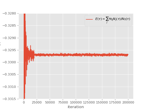
As can be seen, at iteration \(2 \times 10^4\) there is a large reduction in stochastic error.
When performing a blocking analysis, the user should not begin averaging data until after the semi-stochastic adaptation has been turned on, since there is a significant change in the probability distributions of data beyond this point. This is particularly true in initiator FCIQMC simulations, where the use of semi-stochastic can alter the initiator error (although we typically find that semi-stochastic does not alter the magnitude of initiator error significantly, it can in some cases, see [Petruzielo12]). We can therefore analyse the above simulation using
$ reblock_hande.py --quiet --start 30000 hubbard_semi_stoch_high.out
which results in:
Recommended statistics from optimal block size:

                               # H psips \sum H_0j N_j       N_0        Shift   Proj. Energy
hubbard_semi_stoch_high.out  5216460(80)     -15356(2)  46576(5)  -0.32970(2)  -0.3296994(8)
Compared to the equivalent non-semi-stochastic simulation performed in the FCIQMC tutorial tutorial, the error bars on the shift and projected energy estimators have reduced from \(4 \times 10^{-5}\) and \(3 \times 10^{-6}\) to \(2 \times 10^{-5}\) and \(8 \times 10^{-7}\), respectively.
Note that if you do not specify a start_iteration value in the semi_stoch
table of the input file, then the semi-stochastic adaptation will be turned
on from the first iteration. This should not be done when starting a new
simulation, because wave functions in HANDE are initialised as single determinants.
However, if restarting a simulation from an HDF5 file then this is a sensible approach -
the simulation will begin from the wave function stored in the HDF5 file, and the
deterministic space will be chosen from the most populated determinants in this
wave function. An input file for such a restarted simulation would contain the
following semi_stoch and restart tables within the fciqmc table:
fciqmc {
    sys = hubbard_k{...},
    qmc = {...},
    semi_stoch = {
        size = 10000,
        space = "high",
    },
    restart = {
        read = 0,
    },
}
(see the restart options entry in the documentation for more options relating to restarting simulations).
Finally, when restarting simulations which were already using the semi-stochastic
adaptation, it is important to use exactly the same deterministic space to ensure
that estimators are statistically consistent before and after restarting. However,
the approach in HANDE uses the instantaneous FCIQMC wave function to generate the
deterministic space, which changes during the simulation. Using the above approach
would therefore lead to a slightly different space being generated after restarting.
One can get around this by outputting the deterministic space in use to a file, and
reading it back in for the restarted calculation. For example, to generate a
deterministic space from the \(10^4\) most populated determinants at iteration
\(2 \times 10^4\), and to then print this space to a file, one should use the
write keyword in the semi-stoch table:
fciqmc {
    sys = hubbard_k{...},
    qmc = {...},
    semi_stoch = {
        size = 10000,
        start_iteration = 20000,
        space = "high",
        write = 0,
    },
}
Here, the value of the write keyword, \(0\), is an index used in the
name of the resulting file. Note that write can also be a boolean, in which
case HANDE will find and use the smallest unused id available in the directory.
When restarting the simulation, one can then specify the space option to
read a semi-stochastic HDF5 file, using:
fciqmc {
    sys = hubbard_k{...},
    qmc = {...},
    semi_stoch = {
        space = "read",
    },
}
The deterministic space file is an HDF5 file. As such, both writing and reading of such files requires compilation of HANDE with HDF5 enabled, which is the default compilation behaviour.