Solid state calculations
In this tutorial we will run periodic boundary conditions CCMC calculation on a diamond
crystal in STO-3G basis with 2x1x1 sampling of the Brillouin zone. Familiarity with
CCMC and FCIQMC tutorials is assumed.
The input and output files can be found under the documentation/manual/tutorials/calcs/ccmc_solids subdirectory of the source distribution.
First of all, we need the one- and two- electron integrals from an external source. We will use PySCF software package [Sun18] to perform preliminary Hartree-Fock calculation and generate the integrals. PySCFDump script can be used to save the integrals in the FCIDUMP format readable by HANDE [1] .
To correctly address exchange divergence, additional exchange integrals are needed. Those are written in a FCIDUMP_X file by PySCFDump. Theoretical details of this procedure will be elaborated on as part of an upcoming paper.
Cell object can be conveniently prepared using build_cell function of the pyscfdump.helpers
module and ASE library. Set of basis functions, kinetic energy cutoff and pseudopotential
used are specified.
The run_khf function of the pyscfdump.scf module is used to run the HF calculation.
Number of k-points in each dimension is specified. By default, the Monkhorst-Pack grid is used. If
gamma is set to true, the grid will be shifted to include the Gamma point. Exchange divergence
treatment scheme should also be chosen. The function returns the converged HF calculation object
and a list of scaled k-points (i.e. (0.5,0.5,0.5) is at the very corner of the Brillouin zone).
Finally, fcidump function of the pyscfdump.pbcfcidump module is used to dump the integrals
to a file. Name of the resulting file, SCF calculation object, number of k points, list of
scaled k points and boolean variable MP (true if the grid is Monkhorst-Pack - i.e. not shifted to
include the gamma point for even grids) must be provided.
from ase.lattice import bulk
import pyscfdump.scf as scf
from pyscfdump.helpers import build_cell
from pyscfdump.pbcfcidump import fcidump

A2B = 1.889725989	#angstrom to bohr conversion

a=3.567		#lattice parameter
ke=1000		#kinetic energy cutoff in units of rydberg
basis='sto-3g'	#basis set choice
nmp = [2,1,1]	#k point sampling

#prepare the cell object
ase_atom = bulk('C', 'diamond', a=a*A2B)
cell = build_cell(ase_atom, ke=ke, basis=basis, pseudo='gth-pade')

#run the HF calculation
kmf,scaled_kpts = scf.run_khf(cell, nmp=nmp, exxdiv='ewald', gamma=True)

#dump the integrals
fcidump('fcidumpfile',kmf,nmp,scaled_kpts,False)
Now we are ready to run the CCMC calculation. System definition is read in from the FCIDUMP files. There are two points to notice
path to files with additional exchange integrals is specified as
ex_int_fileto properly exploit translational symmetry in the crystal lattice, the orbitals and hence the integrals must be complex. The complex mode of HANDE is enabled by setting
complex = true. Consequently, numbers of particles on excitors also have both real and imaginary part, as well as projected energy.
In a non-initiator calculation, we try setting the time step tau as big as possible before too many blooms happen.
A shoulder plot should be used to determine target_population.
The heat_bath excitation generator [Holmes16] (adapted to HANDE as described in [Neufeld19])
is often a good choice in small systems. The input script used in this tutorial is:
sys = read_in {
    int_file = "fcidumpfile",
    complex = true,
    ex_int_file = "fcidumpfile_X",
}
ex_l=2

ccmc {
    sys = sys,
    qmc = {
        tau = 0.02,
        rng_seed = 13086,
        mc_cycles = 10,
        init_pop = 200,
        nreports = 50000,
        target_population = 1e4,
        state_size = -800,
        spawned_state_size = -500,
        excit_gen = "heat_bath",
        real_amplitudes = true,
    },
    ccmc = {
	even_selection = true,
        full_non_composite=true,
    },
    reference = {
        ex_level = ex_l,
    },
    blocking = {
        blocking_on_the_fly = true,
        auto_shift_damping = true,
    },
    restart = {
        write = true,
    },
}
The Hilbert space of the system we are dealing with is quite small and so is the target population. The general rule is that in order to use MPI parallelism, each process should contain at least \(10^{5}\) occupied excitors [Spencer18]. Having fewer excitors on each process is both inefficient and in extreme cases can lead to biased results. This is why we will use only one process here. However, use of openMP shared memory threads is recommended in order to make full use of the available resources.
$ hande.x ccmc.lua > diamond_ccmc.out
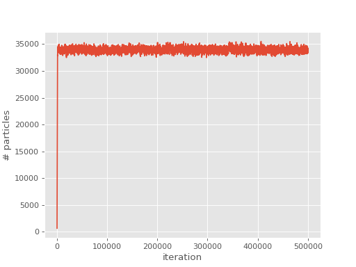
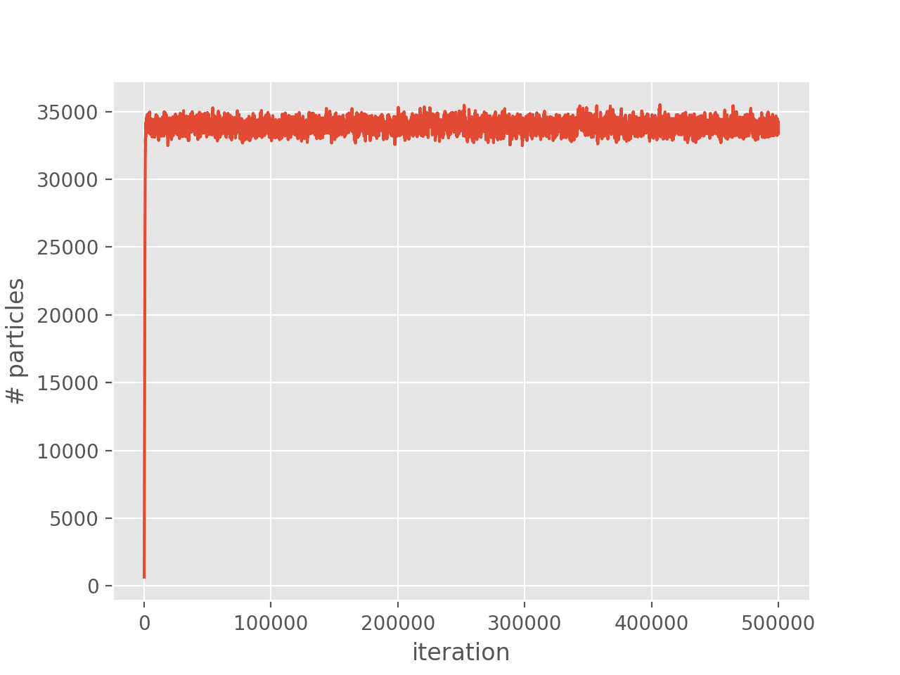
We can now plot the population
(Source code, png, hires.png, pdf)

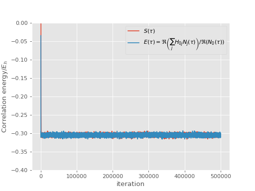
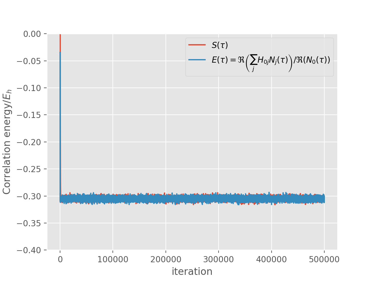
and correlation energy:
(Source code, png, hires.png, pdf)

It is worth noting that the projected energy is in fact a complex quantity, whose imaginary part evaluates to zero in a non-trivial way [Booth13]. For the plot we calculate the result by only using real parts of both \(\sum_j H_{0j} N_j(\tau)\) and \(N_0(\tau)\), using the fact that
\(E(\tau) = \Re\left(\frac{\sum_j H_{0j} N_j(\tau)}{N_0(\tau)}\right) = \frac{\Re\left(\sum_j H_{0j} N_j(\tau)\right)}{\Re\left(N_0(\tau)\right)}\)
where the second equality holds provided that imaginary part of \(E(\tau)\) is zero.
The reblocking analysis uses magnitudes rather than real parts as this prevents problems with potential changes of phase during the calculation. Neverthless, for a well behaved calculation such as the one presented here, it is found that reblocking using real parts would give identical results.
In any case, the shift remains a strictly real measure of the correlation energy [2].
To analyse the calculation we can use reblock_hande.py script:
$ reblock_hande.py --quiet diamond_ccmc.out
which results in:
Block from: 20790
Recommended statistics from optimal block size:

                       Block from  # H psips \sum H_0j N_j      N_0        Shift Proj. Energy
diamond_ccmc_2.out 2.07900000e+04  33940(10)      -1015(2)  3328(6)  -0.30485(8)  -0.30495(5)
Footnotes