Full Configuration Interaction Quantum Monte Carlo

In this tutorial we will run FCIQMC on the 18-site 2D Hubbard model at half filling with \(U/t=1.3\). The input and output files can be found under the documentation/manual/tutorials/calcs/fciqmc subdirectory of the source distribution. Knowledge of the terminology and theory given in [Booth09] and [Spencer12] is assumed.

First, we will set up the system and estimate the number of determinants in Hilbert space with the desired symmetry using a Monte Carlo approach.

We are interested in the state with zero crystal momentum, as there is theoretical work showing this will be the symmetry of the overall ground state. HANDE uses an indexing scheme for the symmetry label. The easiest way to find this out is to run an input file which only contains the system definition:

hubbard = hubbard_k {
    lattice = {
        { 3,  3 },
        { 3, -3 },
    },
    electrons = 18,
    ms = 0,
    U = 1.3,
    t = 1,
}

This file can be run using:

$ hande.x hubbard_sym.lua > hubbard_sym.out

The output file, hubbard_sym.out, contains a symmetry table which informs us that the wavevector \((0,0)\) corresponds to the index 1; this value should be specified in subsequent calculations to ensure that the calculation is performed in the desired symmetry subspace.

It is useful to know the size of the FCI Hilbert space, i.e. the number of Slater determinants that can be formed from the single-particle basis given the number of electrons and total spin. Whilst the full space can be determined from simple combinatorics, the size of the subspace containing only determinants of the desired symmetry is less straightforward and it is the latter number that is of interest as it only includes determinants that are connected via non-zero Hamiltonian matrix elements and hence can be accessed in a Monte Carlo calculation. A fast way to determine the size of the accessible subspace is to use Monte Carlo sampling [Booth10] with an input file containing:

hubbard = hubbard_k {
    lattice = {
        { 3,  3 },
        { 3, -3 },
    },
    electrons = 18,
    ms = 0,
    U = 1.3,
    t = 1,
    sym = 1,
}

hilbert_space {
    sys = hubbard,
    hilbert = {
        nattempts = 100000,
        ncycles = 30,
    }
}

The Monte Carlo algorithm produces nattempts random determinants per cycle, from which it estimates the size of the Hilbert space. The independent cycles are used to provide an estimate of the mean and standard error of the data; the running estimates of these are printed every cycle and the final estimate at the end.

This calculation can be run in a similar fashion to before:

$ hande.x hubbard_hilbert.lua > hubbard_hilbert.out

Inspecting the output, we find that the Hilbert space contains \(1.3 \times 10^8\) determinants with the desired symmetry.

FCIQMC requires a critical population to be exceeded in order to converge to the correct answer. This system-specific population is determined by the plateau. A calculation initially uses a constant energy offset (‘shift’) and a small starting population and hence the population grows exponentially. A plateau in the population growth spontaneously appears, during which the correct sign structure of the ground state wavefunction emerges. The plateau is equally spontaneously exited and the population grows at an exponential rate (albeit slower than the initial growth).

The simplest way to find the plateau is to run an FCIQMC calculation with a small initial population and allow the population to grow until a large size; this can be accomplished by setting target_population, which is the population at which the shift is allowed to vary, to a large value (i.e. effectively infinite) such that the plateau should occur before it. This is done using an input file like [1]:

hubbard = hubbard_k {
    lattice = {
        { 3,  3 },
        { 3, -3 },
    },
    electrons = 18,
    ms = 0,
    U = 1.3,
    t = 1,
    sym = 1,
}

fciqmc {
    sys = hubbard,
    qmc = {
        tau = 0.002,
        mc_cycles = 20,
        nreports = 500,
        init_pop = 100,
        target_population = 10^10,
        state_size = -1000,
        spawned_state_size = -100,
    },
}

As the input file is a lua script, we can use lua expressions (e.g. 10^10 for \(1 \times 10^{10}\)) at any point.

The choice of timestep is beyond the scope of a simple tutorial; broadly it is chosen such that the population is stable and there are no ‘blooms’ (spawning events which create a large number of particles). HANDE will print out a warning and a summary at the end of the calculation if blooms occur. The other key values are how many iterations to run for and the amount of memory to use for the main and spawned particle data objects. These were chosen such that enough states could be stored and the plateau occurs within the iterations used. Choosing these for a new system typically requires some trial and error. Given the large population, we will run this calculation in parallel using MPI:

$ mpiexec hande.x hubbard_plateau.lua > hubbard_plateau.out

The parallel scaling of HANDE depends upon the system being studied and quality of the hardware being used. Typically using a minimum population per core of \(\sim 10^5\) (assuming perfect load balancing, which can rarely be achieved) results in an acceptable performance.

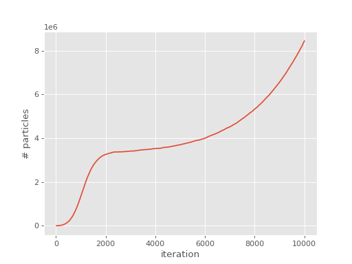
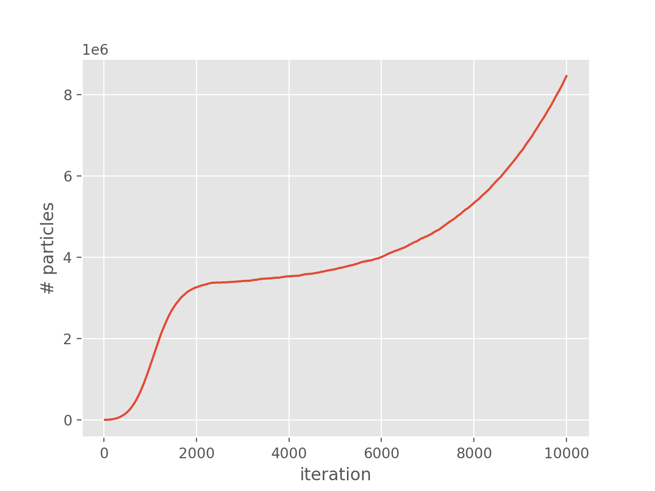
The output file is (hopefully!) fairly intuitive. The QMC output table contains one entry per ‘report loop’ (a set of Monte Carlo cycles). pyhande can be used to extract this information so that the population growth can be easily plotted:

(Source code, png, hires.png, pdf)

We hence see that the plateau occurs at around \(3.5 \times 10^6\) (\(\sim 2.8\%\) of the entire Hilbert space) and hence FCIQMC is very successful for this system.

Note

In some cases the plateau may not be present (e.g. in sign-problem free systems) or not easily visible (e.g. in systems with a small Hilbert space) or appear as a shoulder (common in CCMC calculations). pyhande contains two algorithms for determining the plateau, which are helpful in such cases or for automatically analysing large numbers of calculations.

We can now run a production calculation to find the ground state energy of this system. To do so, we make two changes to the input used to find the plateau: target_population is set to a value above the plateau (but not so large that the computational cost is overwhelming) and the simulation is run for more iterations, i.e.:

hubbard = hubbard_k {
    lattice = {
        { 3,  3 },
        { 3, -3 },
    },
    electrons = 18,
    ms = 0,
    U = 1.3,
    t = 1,
    sym = 1,
}

fciqmc {
    sys = hubbard,
    qmc = {
        tau = 0.002,
        mc_cycles = 20,
        nreports = 10000,
        init_pop = 100,
        target_population = 4*10^6,
        state_size = -1000,
        spawned_state_size = -100,
    },
}

and can again be run using:

$ mpiexec hande.x hubbard_fciqmc_real.lua > hubbard_fciqmc.out

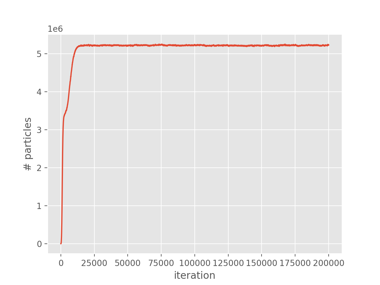
This time, the population starts to be controlled after it reaches the desired target_population:

(Source code, png, hires.png, pdf)

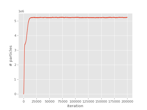
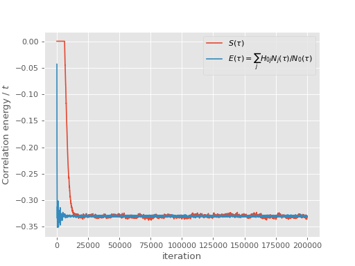
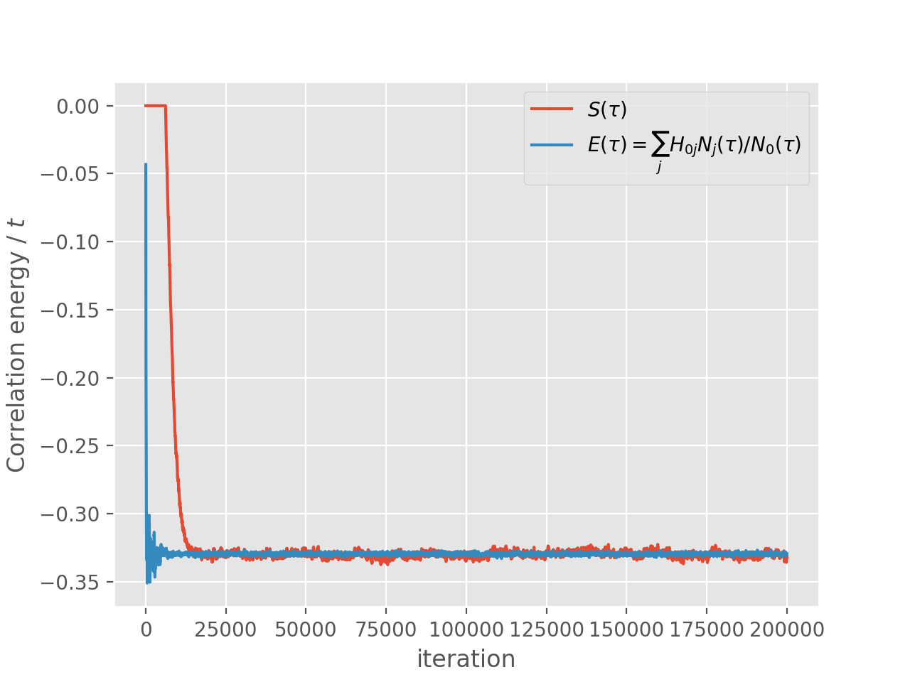
Note that it takes some time for the population to stabilise as the shift gradually decays towards the ground state correlation energy. Once the population is stable, both the shift and the instantaneous projected energy vary about a fixed value, namely the ground state energy:

(Source code, png, hires.png, pdf)

Care must be taken in evaluating the mean and standard error of these quantities, however. The state of a simulation at one iteration depends heavily upon the state at the previous iteration and hence each data point is not independent. Further, in the case of the projected energy estimator, the correlation between the numerator and denominator must be taken into account. The former issue is dealt with using a blocking analysis [Flyvbjerg89]; the latter by taking the covariance into account. Both of these are implemented in pyhande and the reblock_hande.py script provides a convenient command line interface to this functionality. See Analysis for more information. The above graphs show that the popualation, shift and instantaneous projected energy estimator have all stabilised by iteration 30000, so we will accumulate statistics from that point onwards. reblock_hande.py can produce a lot of useful output but for now we’ll only concern ourselves with the best guess of the standard error [Lee11], hence the use of the --quiet flag:

$ reblock_hande.py --quiet --start 30000 hubbard_fciqmc.out

which gives

Recommended statistics from optimal block size:

                               # H psips \sum H_0j N_j        N_0       Shift Proj. Energy
fciqmc/hubbard_fciqmc.out  5222000(1000)      -7791(7)  23630(20)  -0.3299(3)  -0.32969(2)

The stochastic error can be reduced by running with more particles and/or running for longer. Another very effective method is to allow determinants to have fractional numbers of particles on determinants rather than just using a strictly integer representation of the wavefunction. This is done using the real_amplitudes keyword:

hubbard = hubbard_k {
    lattice = {
        { 3,  3 },
        { 3, -3 },
    },
    electrons = 18,
    ms = 0,
    U = 1.3,
    t = 1,
    sym = 1,
}

fciqmc {
    sys = hubbard,
    qmc = {
        tau = 0.002,
        mc_cycles = 20,
        nreports = 10000,
        init_pop = 100,
        target_population = 4*10^6,
        state_size = -1000,
        spawned_state_size = -100,
        real_amplitudes = true,
    },
}

The calculation can be run and analysed in the same manner:

$ mpiexec hande.x hubbard_fciqmc_real.lua > hubbard_fciqmc_real.out
$ reblock_hande.py --quiet --start 30000 hubbard_fciqmc_real.out

which results in:

Recommended statistics from optimal block size:

                                   # H psips \sum H_0j N_j       N_0        Shift  Proj. Energy
fciqmc/hubbard_fciqmc_real.out  5230600(100)     -15460(2)  46890(6)  -0.32976(3)  -0.329694(4)

Whilst using real amplitudes is substantially slower, the reduction in stochastic error more than compensates; it is much more efficient than simply running for longer. Real ampltiudes also reduce the plateau height in some cases (as is the case here) though this has not been investigated carefully in a wide variety of systems.

One reason that the calculation with real ampltiudes took so much longer than that with integer ampltiudes is due to the nature of the Hubbard model: all non-zero off-diagonal Hamiltonian matrix elements are identical in magnitude. Carefully inspecting the output in hubbard_fciqmc_real.out reveals that there is almost one spawning event for every particle [2]. This results in a costly communication overhead every timestep. We can improve this by changing the spawn_cutoff parameter, which is the minimum absolute value of a spawning event [Overy2014]. A spawning event with a smaller cutoff is probabilistically rounded to zero or the cutoff value [3]. The default cutoff value, 0.01, need only be changed in cases such as this and is set using the spawn_cutoff parameter in the qmc table:

hubbard = hubbard_k {
    lattice = {
        { 3,  3 },
        { 3, -3 },
    },
    electrons = 18,
    ms = 0,
    U = 1.3,
    t = 1,
    sym = 1,
}

fciqmc {
    sys = hubbard,
    qmc = {
        tau = 0.002,
        mc_cycles = 20,
        nreports = 10000,
        init_pop = 100,
        target_population = 4*10^6,
        state_size = -1000,
        spawned_state_size = -100,
        real_amplitudes = true,
        spawn_cutoff = 0.1,
    },
}

Note that a value of 1 is comparable to using integer ampltiudes except for the death step, which acts without stochastic rounding if real_amplitudes is enabled.

We can run calculations with different values of spawn_cutoff as before; here we set use values of 0.1, 0.25 and 0.5. reblock_hande.py can analyse multiple calculations at once and so we can easily see the impact of changing spawn_cutoff compared to the default value and the original FCIQMC calculation using integer ampltiudes:

$ reblock_hande.py --quiet --start 30000 hubbard_fciqmc*out

Recommended statistics from optimal block size:

                                           # H psips \sum H_0j N_j        N_0        Shift  Proj. Energy
fciqmc/hubbard_fciqmc.out              5222000(1000)      -7791(7)  23630(20)   -0.3299(3)   -0.32969(2)
fciqmc/hubbard_fciqmc_real.out          5230600(100)     -15460(2)   46890(6)  -0.32976(3)  -0.329694(4)
fciqmc/hubbard_fciqmc_real_sc0.1.out    5225400(200)     -13172(1)   39952(4)  -0.32968(5)  -0.329704(6)
fciqmc/hubbard_fciqmc_real_sc0.25.out   5219300(400)     -10627(4)  32230(10)   -0.3298(1)  -0.329696(9)
fciqmc/hubbard_fciqmc_real_sc0.5.out    5220500(600)      -9595(4)  29100(10)   -0.3296(2)   -0.32970(1)

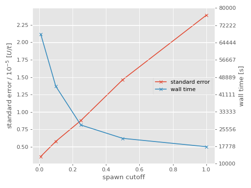
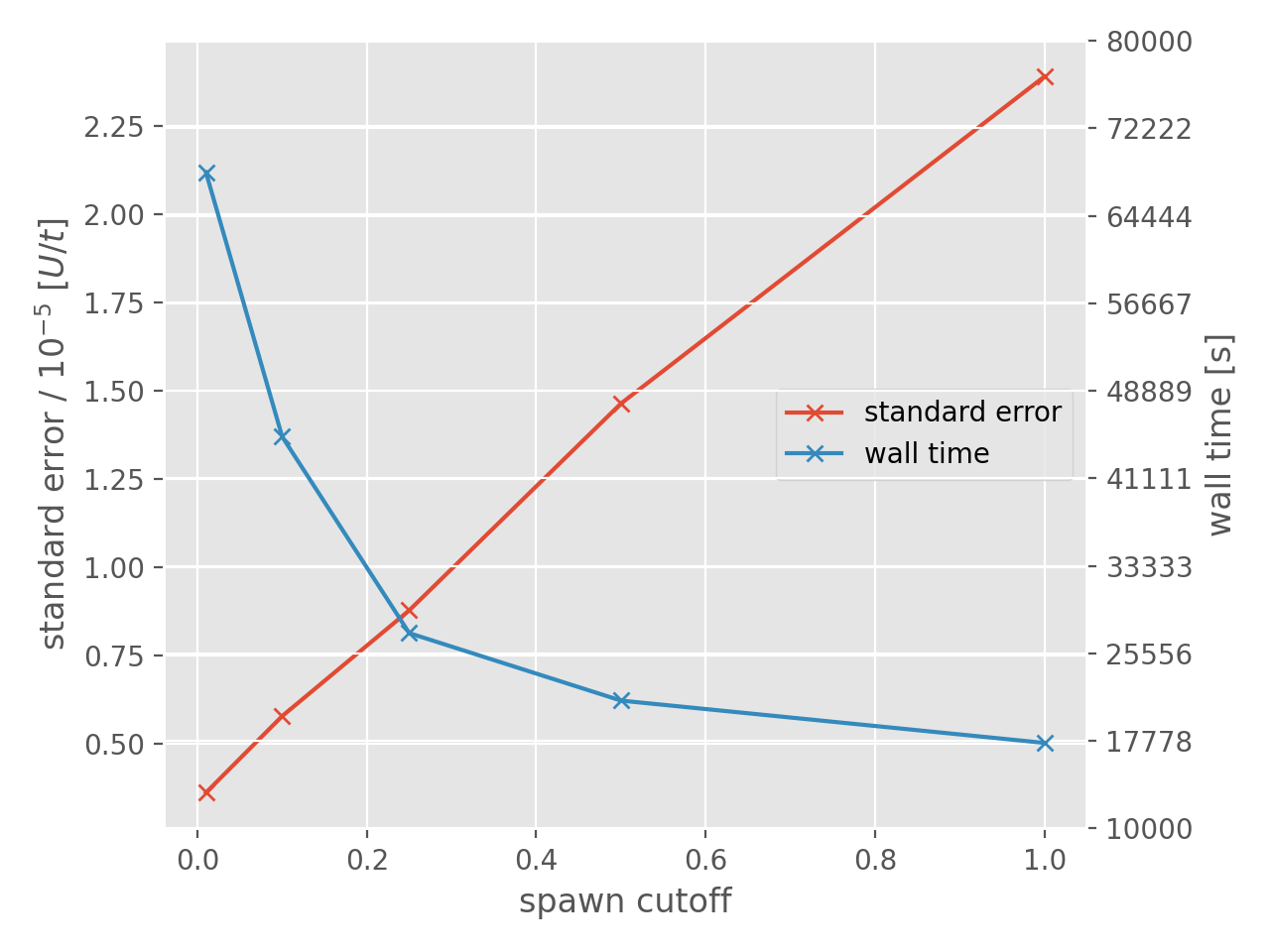
As expected, increasing the spawn_cutoff results in an increase in the stochastic error (linear, in this case, due to the identical magnitude of non-zero off-diagonal Hamiltonian matrix elements). Finally, we can compare the change in stochastic error to the wall time of the calculation:

(Source code, png, hires.png, pdf)

For convenience, the integer amplitude calculation is shown as having a spawn_cutoff of 1. Clearly there is a playoff between the computational cost and the desired stochastic error; choosing a value of 0.25 for spawn_cutoff in this case seems sensible as it is around the point where the rate of change in the wall time begins to slow [4].

Footnotes

[1]	With some scripting it is possible to automatically detect the plateau and interact with the calculation at this point.

[2]	This can be confirmed analytically using knowledge of the internal excitation generators and the associated probabilities, the value of \(U/t\) and the calculation timestep.

[3]	One can hence view the integer amplitudes algorithm, ignoring death and spawning events which produce multiple particles, as having a spawn_cutoff of 1.

[4]	A more comprehensive approach to assessing the efficiency of the calculations can be found in [Vigor16].