Shoulder Plots
This tutorial looks further into finding the optimal target particle population in more detail. It is advisable to have read the FCIQMC and CCMC tutorials before this one. More information and details on shoulder plots can be found in [Spencer15].
The example used here is a CCSDT Monte Carlo calculation on water in a cc-pVDZ basis [Dunning89].
As in the CCMC tutorial, the integrals were calculated with PSI4
(see Generating integrals for details). Input and output files are in documentation/manual/tutorials/calcs/shoulder/.
The first calculation was run using
sys = read_in {
    int_file = "H2O_INTDUMP",
    nel = 10,
    ms = 0,
}

ccmc {
    sys = sys,
    qmc = {
        tau = 1e-4,
        mc_cycles = 10,
        nreports = 2e4,
        state_size = -500,
        spawned_state_size = -200,
        init_pop = 200,
        real_amplitudes = true,
	target_population = 3e5,
    },
    reference = {
        ex_level = 3,
    },
}
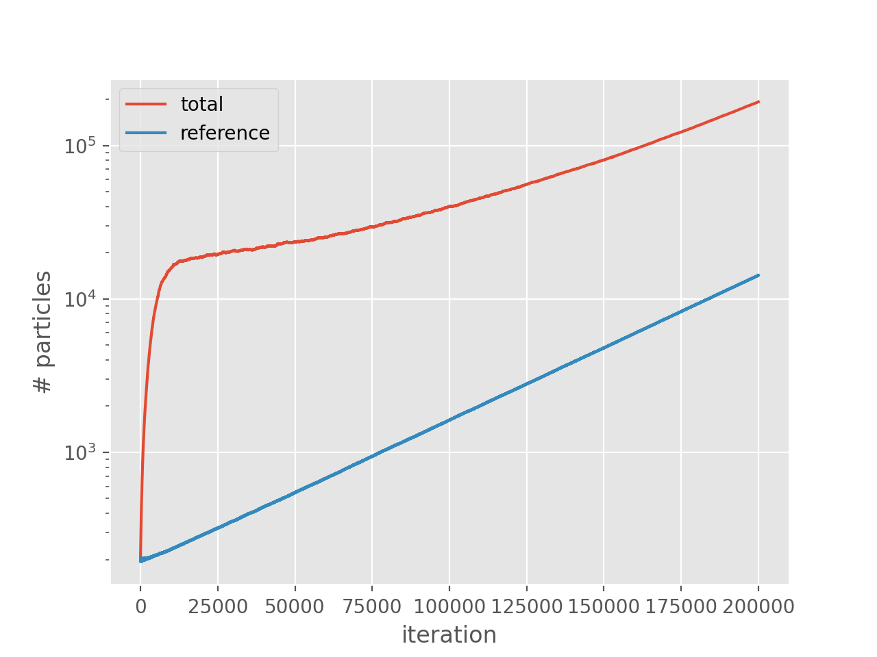
Just like FCIQMC, a plateau can be seen in a total population vs iteration plot, which indicates roughly the minimum particle number to make the calculation stable:
(Source code, png, hires.png, pdf)
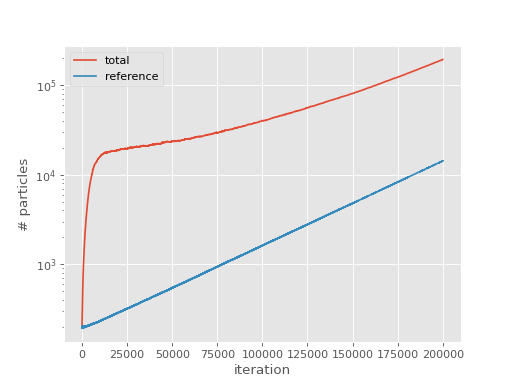
The plateau is clearly visible at around 20000 particles. This is one technique but the plateau is frequently not so easy to observe by visual inspection, especially for CCMC and being able to estimate it computationally is useful for analysing large numbers of calculations.
In the beginning of a typical simulation, only the reference is occupied. Its particles then spawn to occupy parts of the remaining Hilbert space, making the total population grow at a greater pace than the population on the reference does. At the plateau point, annihilation, spawning and death balance each other which temporarily leads to a constant total population while the reference population keeps growing. After a bit, the total population grows again and leaves the plateau. It then grows at a smaller or the same rate as the reference population because the system is now converged and the distribution of particles stochastically represents the ground state wavefunction of the system. See [Spencer12] and [Spencer15] for details.
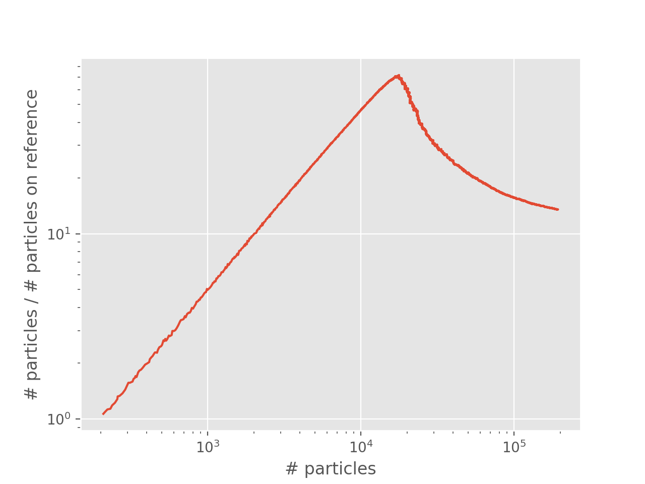
The ratio of total population to population on the reference therefore peaks at roughly the plateau with respect to the total population. A good way to find the position of the plateau is therefore to look at the ratio of total population to population on the reference vs total population plots and find the position of the peak. We call this “shoulder” plot and the peak, or “shoulder height”, is an upper limit for the position of the plateau, see [Spencer15]. The shoulder plot for our example from above is:
(Source code, png, hires.png, pdf)

The position of the shoulder is at about 20000 which corresponds to the position of the plateau.
Note
pyhande contains two functions to estimate the position of the
plateau/shoulder: pyhande.analysis.plateau_estimator(), which looks
for the peak in the shoulder plot [Spencer15], and pyhande.analysis.plateau_estimator_hist(),
which uses a histogram approach to identifying the plateau [Shepherd14]. As a result
of the difference in approaches, the former tends to pick up the population at the
start of the plateau whilst the latter favours the end of the plateau and is less well
suited to cases without a clear plateau.
In this case, plateau_estimator gave 18481 with an estimated standard error of 38
for the shoulder height and plateau_estimator_hist gave 20155 (rounded to 0 d.p.).
The difference is not important as the plateau is not exactly constant; its value to a
few significant values is the important quantity.
The position of the plateau/shoulder is somewhat sensitive to input parameters and can be
varied with changing the time step tau or the cluster_multispawn_threshold (if
applicable) for example, more details below. A large initial population init_pop can
also lead to overshooting of the shoulder.
Effects of the Time Step
Now we will run another calculation with a higher time step, see input file below:
sys = read_in {
    int_file = "H2O_INTDUMP",
    nel = 10,
    ms = 0,
}

ccmc {
    sys = sys,
    qmc = {
        tau = 1e-3,
        mc_cycles = 10,
        nreports = 3.6e3,
        state_size = -500,
        spawned_state_size = -200,
        init_pop = 200,
        real_amplitudes = true,
	target_population = 3e5,
    },
    reference = {
        ex_level = 3,
    },
}
The two resulting shoulders are shown in the following graph:
(Source code, png, hires.png, pdf)
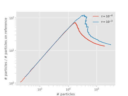
A smaller time step can lead to fewer particles at the shoulder position, as described in [Booth09], [Vigor16].
Effects of Cluster Multispawn Threshold
This part looks at changing the multispawn threshold. This is another feature which can change the number of particles at the shoulder. Positive effects of that have already been shown in CCMC. Note that while changing the time step changes the position of the plateau for FCIQMC for example as well, cluster multispawn threshold is specific to CCMC. The lower the multispawn threshold, the lower will be the number of “blooming” events which spawn multiple particles at the same spawning attempt. “Blooming” events can lead to greater uncertainty as the wavefunction is then sampled in a more coarse and less fine manner. It is therefore not surprising that less particles are needed to converge to the correct wavefunction for a lower multispawn threshold.
To demonstrate the effects of decreasing the multispawn threshold, we will run the following calculation with a low multispawn threshold:
sys = read_in {
    int_file = "H2O_INTDUMP",
    nel = 10,
    ms = 0,
}

ccmc {
    sys = sys,
    qmc = {
        tau = 1e-4,
        mc_cycles = 10,
        nreports = 2e4,
        state_size = -500,
        spawned_state_size = -200,
        init_pop = 200,
        real_amplitudes = true,
	target_population = 3e5,
    },

    ccmc = {
	cluster_multispawn_threshold = 0.1,
    },

    reference = {
        ex_level = 3,
    },
}
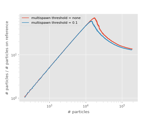
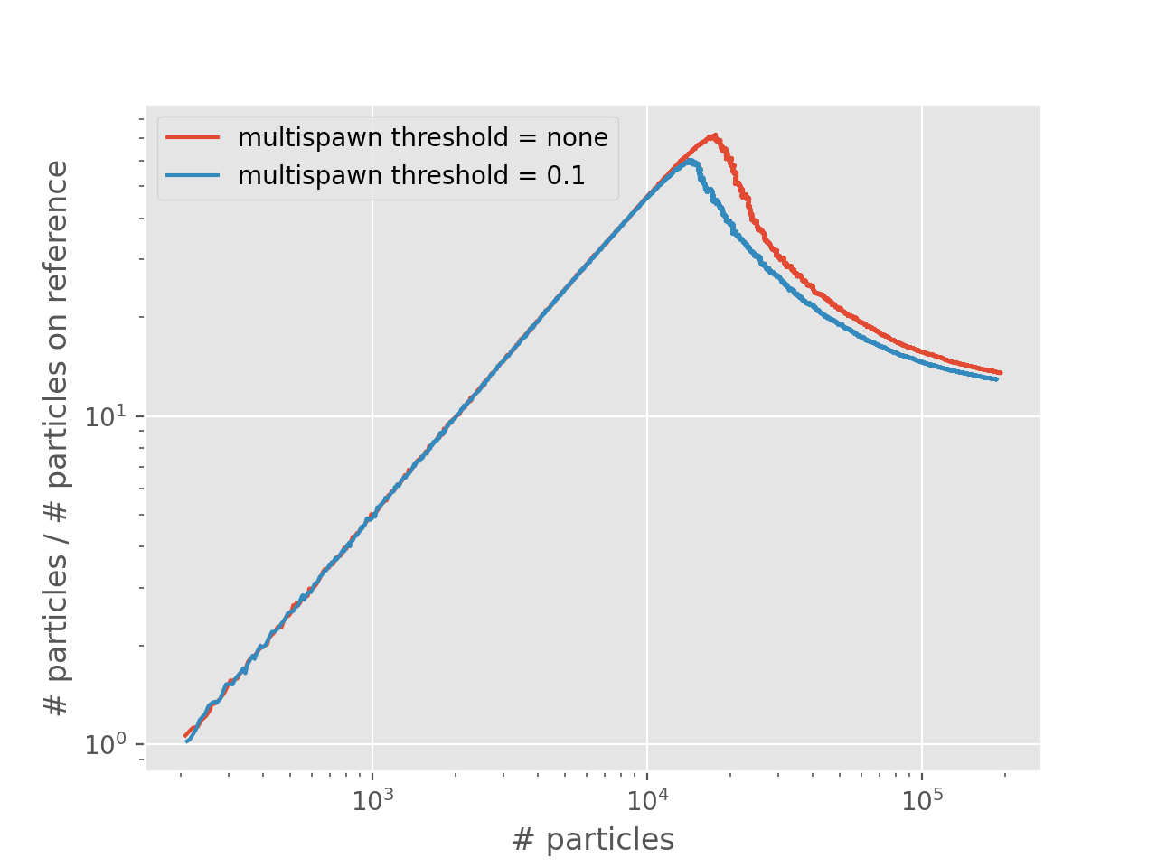
The plot below compares the shoulder plot of this and the first calculation on top of this tutorial:
(Source code, png, hires.png, pdf)

Note that “multispawn threshold = none” means that there is no threshold within computer number representation limits.
Clearly, setting a low multispawn threshold lowers the total number of particles at the shoulder. This is, like with a smaller timestep, due to more efficient sampling: an excitor with a large amplitude is allowed to explore more of the space (via multiple spawning attempts) than an excitor with a smaller amplitude.
Effects of Initial Population
In this part of the tutorial we will see that a large initial population can lead to overshooting the shoulder.
As a demonstration, we look at almost the same calculation as the first one but with a larger initial population.
sys = read_in {
    int_file = "H2O_INTDUMP",
    nel = 10,
    ms = 0,
}

ccmc {
    sys = sys,
    qmc = {
        tau = 1e-4,
        mc_cycles = 10,
        nreports = 2e4,
        state_size = -500,
        spawned_state_size = -200,
        init_pop = 800,
        real_amplitudes = true,
	target_population = 3e5,
    },
    reference = {
        ex_level = 3,
    },
}
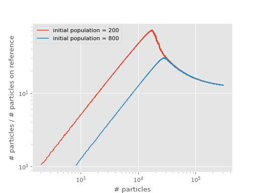
The following plot compares the original with the calculation starting with a large initial population:
(Source code, png, hires.png, pdf)

We see that the calculation with a larger initial population has a shoulder at a larger number of particles, effectively overshooting the shoulder. At yet larger numbers of particles than this, we expect the calculation to be stable once population control is enabled (i.e. the shift is allowed to vary).
The overshooting can be explained by considering that the only significant difference between the two curves above is that they start with a different population at the reference. Before they reach a shoulder, each calculation has a very fast growth in total population without changing the reference population. This results in an initial linear growth on the shoulder plots, which lasts until the reference populations begin to grow.
The calculation with the greater initial population will require a greater total population to reach this point, and it occurs when this calculation’s curve hits that which begins with a smaller population.
Once a calculation has passed its shoulder, the location on the shoulder plot can generally be used to describe its ‘state’. Two calculations with different initial populations, but otherwise identical, will end up on the same curve once equilibrated, and will follow the curve if total particle numbers are allowed to grow. Modifying the algorithm (e.g. with multispawn_threshold) or changing the timestep will cause the equilibrium curve to shift position, and therefore affect the position of the shoulder.