Initiator Approximation to FCIQMC
We shall again calculate the ground state energy of the 18-site 2D Hubbard model at half-filling and with \(U/t=1.3\), as in the FCIQMC tutorial. The initiator approximation [Cleland10] greatly reduces the number of particles required to sample the wavefunction. The drawback, however, is that the approximation must be carefully controlled to obtain an accurate estimate of the FCI energy by running multiple calculations with increasing populations.
It is efficient (both computationally and in terms of elapsed time) to treat each
calculation separately. For compactness, we shall simply run multiple calculations with
different target_population values one after the other in the same HANDE calculation.
This is trivial to do by using a lua loop as fciqmc is simply a function call:
hubbard = hubbard_k {
    lattice = {
        { 3,  3 },
        { 3, -3 },
    },
    electrons = 18,
    ms = 0,
    U = 1.3,
    t = 1,
    sym = 1,
}

targets = {2.5*10^3, 5*10^3, 7.5*10^3, 10^4, 2.5*10^4, 5*10^4, 1*10^5, 2.5*10^5, 5*10^5, 1*10^6}
for i,target in ipairs(targets) do
    qmc_state = fciqmc {
        sys = hubbard,
        qmc = {
            tau = 0.002,
            mc_cycles = 20,
            nreports = 10000,
            init_pop = 100,
            target_population = target,
            state_size = -1000,
            spawned_state_size = -100,
            initiator = true,
        },
    }
    -- For memory efficiency, explicitly free qmc_state after each calculation.
    qmc_state:free()
end
The only difference between the above input and an FCIQMC calculation is the setting
initiator = true. As in the examples in the FCIQMC tutorial,
this can be run using:
$ mpiexec hande.x hubbard_ifciqmc.lua > hubbard_ifciqmc.out
Again, the exact command to launch MPI will vary with MPI implementation and local configurations.
Inspecting the output, we see one iFCIQMC
calculation was run for each call to the fciqmc function. pyhande
(and, by extension, reblock_hande.py) can handle such cases, so we easily extract and
inspect the data for each calculation.
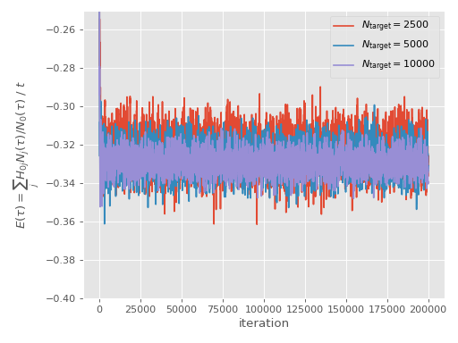
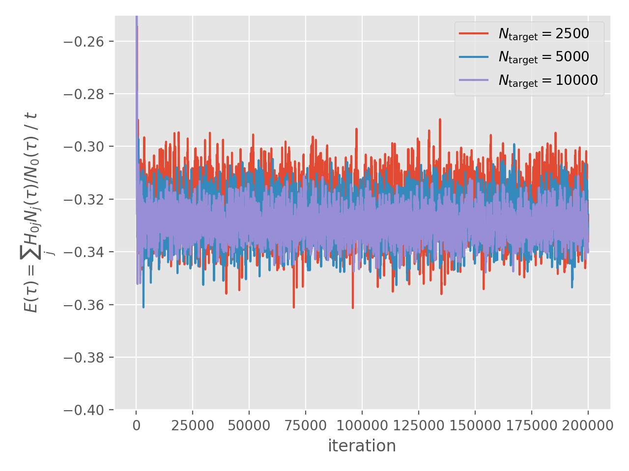
Let’s start by inspecting instantaneous projected energy estimator for the three smallest populations:
(Source code, png, hires.png, pdf)

Whilst the difference is small on this scale, it is evident that the calculation with the
smallest population has a slightly higher mean than calculations with larger populations.
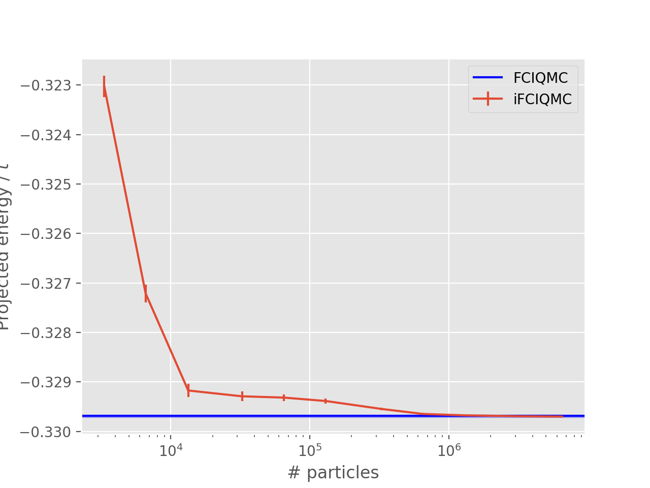
To confirm this, we will plot the energy as a function of population. As
target_population is the population at which the population starts to be
controlled, we should consider the average population (which is somewhat higher).
We can also compare directly to the FCIQMC energy in this case, as the population required
for the FCIQMC calculation is sufficiently small:
(Source code, png, hires.png, pdf)
The light blue region indicates the extent of the FCIQMC stochastic error, as calculated in the FCIQMC tutorial. In this case, the initiator approximation reduces the population required by a factor of \(\sim 2\). However, many studies (including on the electron gas and molecular systems) have demonstrated the initiator approximation can reduce the population required by many orders of magnitude.
The estimates for each calculation can be found directly by using reblock_hande.py:
$ reblock_hande.py --quiet --start 30000 hubbard_ifciqmc.out
where again we chose the start point from inspecting the population growth. This gives:
Recommended statistics from optimal block size:

                                   # H psips \sum H_0j N_j         N_0        Shift  Proj. Energy
ifciqmc/hubbard_ifciqmc.out 0        3332(6)      -91.6(1)    283.6(4)    -0.325(2)    -0.3230(2)
                            1        6609(9)     -153.6(2)    469.4(8)    -0.328(2)    -0.3272(2)
                            2      13360(10)     -293.3(3)    890.9(7)    -0.329(1)    -0.3292(1)
                            3      32580(20)     -718.7(4)     2182(2)   -0.3293(6)    -0.3293(1)
                            4      65230(30)    -1403.2(6)     4261(2)   -0.3291(5)   -0.32932(7)
                            5     130170(30)    -2586.4(5)     7853(2)   -0.3289(3)   -0.32939(5)
                            6     326320(60)    -5520.8(8)    16753(3)   -0.3298(2)   -0.32955(3)
                            7     651010(80)      -9937(1)    30146(4)   -0.3296(1)   -0.32965(2)
                            8   1318400(100)     -19354(2)    58707(6)  -0.32969(9)   -0.32968(2)
                            9   3279800(200)     -48971(4)  148530(20)  -0.32962(7)  -0.329693(8)
                            10  6512700(200)     -97670(4)  296240(10)  -0.32971(5)  -0.329700(7)
reblock_hande.py can also handle the case where each calculation is run separately and
each separate file is passed in as a separate argument on the command line.
Note
We highly recommend a visual inspection of the plot of the initiator error as a function of population as the convergence can be non-monotonic and, as a result, at least two calculations at different populations with statistically equivalent results are required in order to confirm the error due to the initiator approximation is smaller than the stochastic error.
Finally, using real populations can, as with the FCIQMC tutorial, have
a significant impact on the stochastic error. Again, this is done by setting
real_amplitudes = true in the input file (see
hubbard_ifciqmc_real.lua). We also
choose to set spawn_cutoff to 0.25 following the investigation in FCIQMC
tutorial; this results in a small increase in the stochastic error but
results in the calculation taking roughly half the time. Again, note this is somewhat
unique to the Hubbard model. Running:
$ mpiexec hande.x hubbard_ifciqmc_real.lua > hubbard_ifciqmc_real.out
followed by the blocking analysis on the output:
$ reblock_hande.py --quiet --start 30000 hubbard_ifciqmc_real.out
results in
Recommended statistics from optimal block size:

                                        # H psips \sum H_0j N_j         N_0        Shift  Proj. Energy
ifciqmc/hubbard_ifciqmc_real.out 0        3271(2)     -91.03(5)    280.7(2)   -0.3234(9)    -0.3243(1)
                                 1        6643(4)    -148.28(8)    451.5(3)   -0.3298(7)   -0.32844(7)
                                 2       13100(7)     -288.8(2)    877.4(7)   -0.3285(7)   -0.32917(7)
                                 3       32762(7)     -744.6(2)   2261.7(7)   -0.3290(3)   -0.32925(5)
                                 4      65570(20)    -1510.1(4)     4586(1)   -0.3300(3)   -0.32930(3)
                                 5     130830(20)    -2855.0(3)     8669(1)   -0.3295(1)   -0.32934(2)
                                 6     326640(30)    -5821.8(6)    17665(2)   -0.3296(1)   -0.32957(1)
                                 7     660180(40)   -10118.3(5)    30694(2)  -0.32981(7)   -0.32965(1)
                                 8    1303850(60)     -19413(1)    58882(4)  -0.32958(5)  -0.329689(8)
                                 9    3287160(90)     -51020(2)   154749(5)  -0.32969(3)  -0.329699(5)
                                 10  6548200(100)    -103229(2)  313100(10)  -0.32967(2)  -0.329698(3)
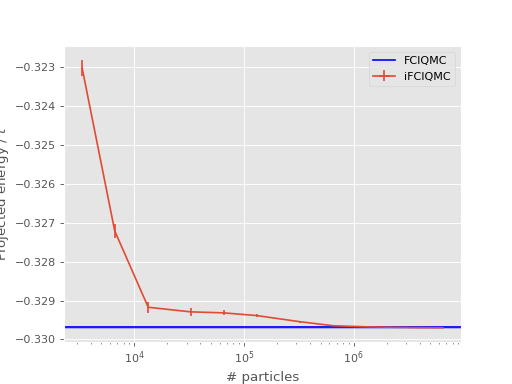
Again, there is a general trend (though not entirely smooth) for the energy estimators to converge to the same energy as a function of total population. It is interesting to take a close look at the convergence of the projected energy estimator:
(Source code, png, hires.png, pdf)
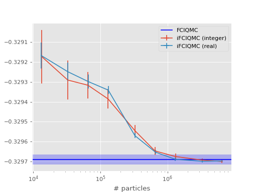
The cluster of results around populations of \(5\times10^5\) shows that it is vital to reduce the stochastic error before deciding the remaining initiator error is negligible. Further, it is interesting to note that the initiator approximation results in a much more efficient sampling of the Hilbert space: for a similar population (\(\sim10^6\)), the iFCIQMC calculations have a much smaller stochastic error for a similar computational cost.